ggplot commands are good for 99% of figure customizations, but sometimes you need to edit individual plot components manually. Here’s how.
R
ggplot
dataviz
Author
Max Czapanskiy
Published
October 20, 2023
I’m working on the figures for a community ecology study and I want to use the same color scheme for the three communities in both geometries and text. It’s easy to assign colors to geometries, but can be harder for text. In this example, I have a bar plot faceted by community, and I want the strip labels to match the colors I use to represent the communities in other figures.
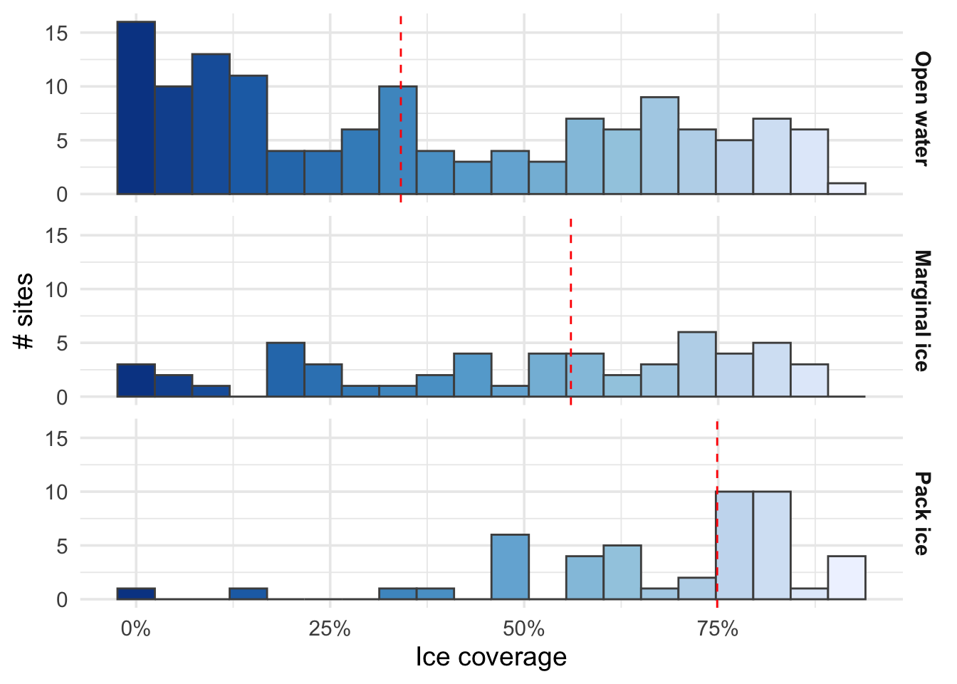
Now we create the figure without color-coding text. From top to bottom, we have three communities (Open water, Marginal ice, and Pack ice) and their sea ice coverage associations. In my other figures I’ve color-code their geometries as green, orange, and purple. I’d like to make my facet strip labels use the same colors here.
ggplot will let me format all the facet strip labels using theme(), however individually formatting them is unsupported (as far as I’m aware). So we’re going to look into the ggplot object’s guts and manually adjust things. Here’s how that works.
Force ggplot to generate the plot
Calling ggplot() only defines the plot at a relatively high level. We need ggplot to actually generate all the plot elements (axes, geometries, legends, etc) before we can start mucking around with them. We do that by calling the grid package’s grid.force() on the plot’s grob (ggplot lingo for a graphical object).
g <- p %>%ggplotGrob() %>%grid.force()
Notice ggplot and grob objects are different classes.
class(ggplot())
[1] "gg" "ggplot"
class(ggplotGrob(ggplot()))
[1] "gtable" "gTree" "grob" "gDesc"
Find the relevant grobs
Now we can look inside to see how ggplot is rendering the facet strip labels and start changing the graphical parameters (like color). The grobs within the plot are arranged in a tree-like structure. For example, legend labels are part of the legend are part of the overall layout. So each grob has both a name (the leaf of the tree) and a path (the sequence of branches leading to the leaf). Extract those like this.
# Get the names and paths of grobsgrob_ls <-grid.ls(g, print =FALSE)grob_names <- grob_ls$namegrob_paths <- grob_ls$gPath
If you examine grob_paths you’ll get an idea of how the paths are structured. Here we see 18 grobs contain the word “strip” in the path. I’ve appended the grob names at the end to show the grob leaf and branches together.
These grobs include the three strip parents ([1], [7], and [13]), each of which has multiple children. The grob that actually contains the graphical parameters we want to edit have name like “GRID.text.*” (which I only figured out through trial and error, that’s not immediately obvious).
Edit the grobs
Knowing where the grobs we want to change are, we can change their graphical parameters.
# This gets the names of the GRID.text grobs for the strip titlesstrip_names <-str_subset( grob_names[str_detect(grob_paths, "strip.text.*titleGrob")],"GRID.text")# I want to change the colors of the strip titles to match the Dark2 palettetxt_colors <- RColorBrewer::brewer.pal(3, "Dark2")for (i in1:3) {# THIS IS THE KEY PART g <-editGrob(grob = g,# Even though the parameter is called gPath, you just give it# the grob's name.gPath = strip_names[i], # Use gpar() to change the graphical parametergp =gpar(col = txt_colors[i]))}
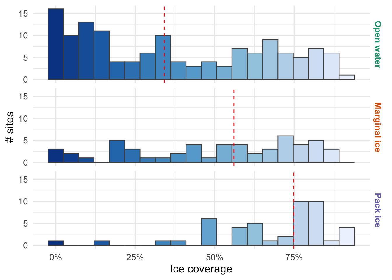
Success!
Now the colors of my strip label text match the other figures in my paper.